Statistics with M&Ms, Part III: Setting good priors

Overview

Teaching: 0 min
Exercises: 0 min

Questions

• How can we design an informative prior for the M&Ms problem?

Objectives

• First learning objective. (FIXME)

In the previous episode, we’ve talked extensively about the likelihood. In the exercises and the discussion of that episode, we’ve just asserted that we know what the fraction of blue M&Ms that are produced at a factory is. In reality, we don’t. This is what we are trying to compute using Bayes’ rule.

To do that, we need another ingredient: we need the prior. While most of us probably don’t have a friend who works at a factory producing M&Ms who could tell us how much blue food colouring they use, we are probably not entirely without knowledge. In most problems we are trying to figure out by using data, we don’t work in a vacuum: there have been studies about that problem before ours, or measurements for a similar problem that influence our approach to the problem, and often also the parameters we are trying to infer.

Bayesian statistics gives you a convenient way to encode that knowledge mathematically via a prior probability distribution. This is a distribution for the parameters we are trying to estimate, before we’ve seen the data.

Priors

In general, don’t use your data to estimate what your priors should be! This would mean you would use the data twice: once to figure out the prior, and once in the likelihood. In reality, this often makes you more confident about your parameter values than you should be.

Exercise: Priors for the M&M problem

What do you know about M&Ms? How many colours are there in a bag? How do you think they’re distributed? Think about this for a few minutes, then discuss with your neighbour.

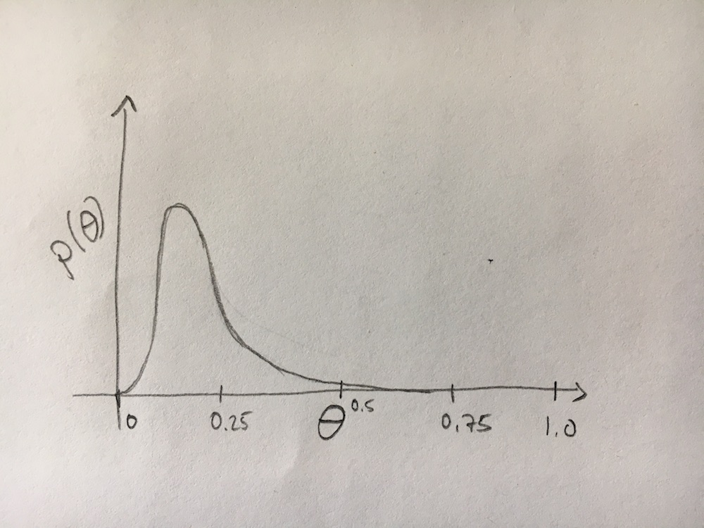
Draw an idea of what you think the prior probability distribution might look like on a piece of paper, and share with your neighbour (and the group).

Reminder: Our parameter, $\theta$, describes the fraction of blue M&Ms in a bag. That fraction naturally goes from 0 (no blue M&Ms) to 1 (all M&Ms are blue). Draw a graph of how probable you think the different values of $\theta$ between 0 and 1 are. Which values do you think are particularly probable? Which are particularly improbable?

Solution

Each bag of M&Ms has six different colours: red, orange, yellow, brown, green and blue. Since we know that there are blue M&Ms, this pretty much excludes the value 0. Because we also know that there are six colours, this also mostly excludes the value 1.

Naively, it might not be a bad assumption that all colours are equally present. This would mean that the fraction of M&Ms that are blue should be around $1/6 = 0.167$. But we don’t know that this is the correct fraction, so we should leave some wiggle room that it could be larger or smaller, though probably not very large and not very small.

Here’s a (badly drawn) graph of what that might look like:

So what should the form of the distribution be? We think it should somehow peak near 0.167, and it should fall off as we go away from that value, but how do we write that down mathematically?

There a number of distributions that could do what we need it to do (for example, a normal distribution with a mean of 0.167 might be a reasonable prior), so how to choose?

The good news are that if our data set is of high enough quality, the prior does not matter very much. This is because we multiply the prior and the likelihood together, so if the prior is wrong (for example, because really 80% of all M&Ms are blue), but we’ve collected thousands of M&Ms and recorded their colours, then the likelihood will be very peaked at the correct value, overwhelming whatever wrong estimates we’ve made in the prior.

However, the flip side of this is that when our data is not very informative about the problem, the prior might actually determine what our posterior probability distribution looks like. This is something that opponents of Bayesian statistics don’t like very much, because of the subjectivity that might be introduced when we choose a prior. However, Bayesians would counter that this just reflects our knowledge of the world, and our uncertainty about it.

Conjugate Priors

So we have a basic idea for what the shape of our prior should be, but we need to parametrize it into an actual mathematical equation we can use. There is a particular class of priors that are very handy in practice because they make calculations straightforward.

One big drawback of Bayesian statistics is that the posterior probability distribution is often not something you can write down analytically. This is because usually the likelihood is some complicated function, and the prior might also be a complicated function, and multiplying these two together leads to an even more complicated function that you can only evaluate numerically. There are a lot of clever algorithms to do that (one very popular one is Markov Chain Monte Carlo), but for today’s exercise, it would be great to have something simpler.

There’s a class of priors that helps with that: they are called conjugate priors, and they describe priors that, when multiplied with a certain likelihood, again give you an analytically function for the posterior. Different likelihood functions have different conjugate priors. Wikipedia has a nice list of conjugate priors for different typical probability distribution that are often used as likelihoods.

In that list, we can find the binomial distribution, for which the conjugate prior is the beta distribution, defined as:

Here, $\alpha$ and $\beta$ are parameters that describe the shape of the distribution. In statistics, they are often called hyperparameters to distinguish them from the parameters we are trying to estimate ($\theta$). In order to use this prior distribution, we need to set reasonable values for $\alpha$ and $\beta$ that produce a shape that is close to what we think the prior for the fraction of blue M&Ms should be.

The Beta Distribution.

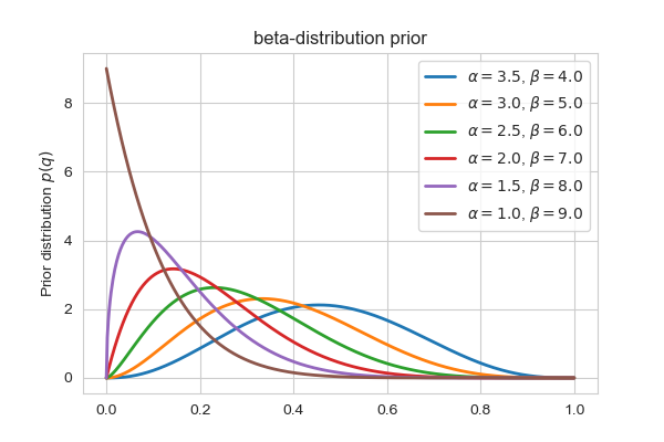
Like the binomial distribution, the beta distribution is implemented in scipy.stats. Plot values of this distribution between 0 and 1 for different values of $\alpha$ and $\beta$. For which values of the hyperparameters does the distribution look like your hand-drawn version?

Solution

Let’s write a loop that goes through some values for $\alpha$ and $\beta$ and plots the beta-distribution between 0 and 1:

fig, ax = plt.subplots(1, 1, figsize=(6,4))

qtrial = np.linspace(0, 1, 500) # trial values of q

alpha = [3.5, 3, 2.5, 2., 1.5, 1]# set the value for alpha
beta = [4,5,6,7,8,9]# set the value for beta

for a, b in zip(alpha, beta):
    # set up the probability distribution
    beta_dist = scipy.stats.beta(a, b)

    # calculate the probability density for qtrial
    beta_pdf = beta_dist.pdf(qtrial)
    

    # plot the results
    ax.plot(qtrial, beta_pdf, lw=2, label=r"$\alpha=%.1f$, $\beta=%.1f$"%(a,b))
    ax.set_label(r"Parameter $q$")
    ax.set_ylabel(r"Prior distribution $p(q)$")
    ax.set_title("beta-distribution prior")
    
plt.legend()

Here’s what the resulting plot looks like:

From this plot, it looks like $\alpha = 2$ and $\beta = 7$ looks similar to what we think the prior for the blue M&M fraction should look like.

Key Points

• First key point. Brief Answer to questions. (FIXME)