Decision Boundaries

Overview

Teaching: 5 min
Exercises: 15 min

Questions

• How can we tell whether the features we have recorded for our samples are good at separating the different classes?

• How can we build visual representations of our features?

Objectives

• Learners understand the relevance of different features for the success of classification.

• Learners understand the concept of a decision boundary and how to draw one.

Now that we have recorded some features for our training data set, how do we go from features to classifying new data points? We’re ready to learn our first algorithm!

In supervised machine learning, which is what we are going to do here, one uses the training data to adjust the model (or algorithm) such that it classifies any new samples as accurately as possible. There are many new concepts and complications hidden in that statement, but we’ll break them down one by one.

Decision Boundaries

First, let’s see how well our features separate different types of candy. We will draw a figure of our features on a large sheet of paper and then place candy into the appropriate areas defines by these features. This will allow us to see how some types of candies might cluster together.

Challenge: Making Plots of Features

For this exercise, we are going to make plots of our features using the candies.

1. First, pick two of the features you defined and gathered data for in the previous lesson.
2. Now take a large sheet of paper, and draw two perpendicular axes. Label them according to the features you selected.
3. Look at your data and find the minimum and maximum for each feature across all of our training data set, then label the axes such that it spans the full range of your data set.
4. Place your different candies in different places on your graph, depending on their values of the features you selected. For this exercise, you don’t need to identify each candy with the appropriate row: just place them approximately in the right place. If you don’t have candies in front of you, you can look at the data from the last lesson in this file, and mark on the paper where the candy should be.

Now take some observational notes while you answer these questions:

• What do you see? Do your candies all end up in different corners of the graph? Are some of them squashed together?
• Compare your results with your neighbour’s. Did you pick similar features? Why not? How are your graphs different?

Solution

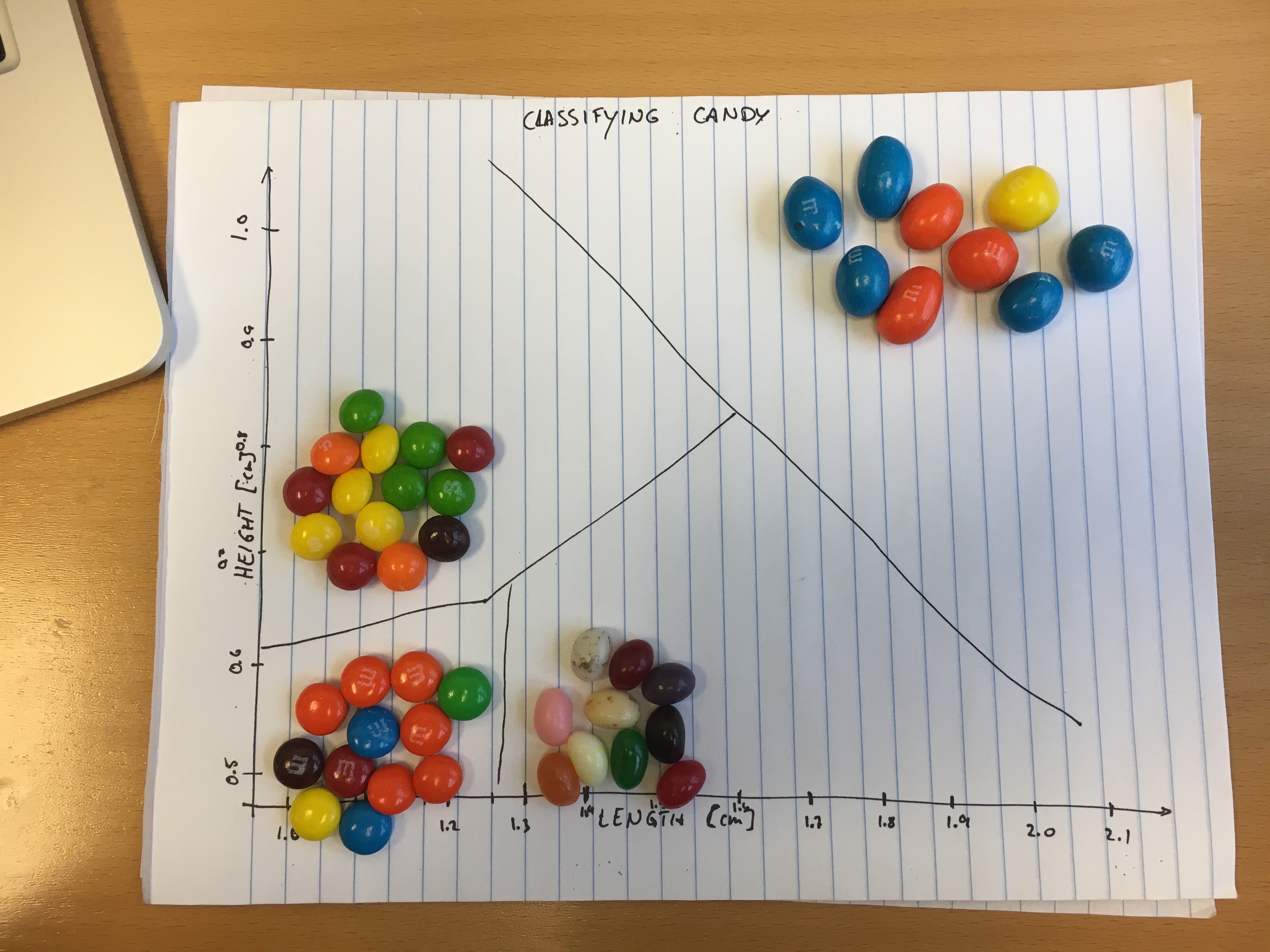
For this solution, I’m going to look at the length of a candy compared to its height. That is, if you let it lie on an even surface, I’m going to measure the longest horizontal axis, and the vertical axis away from the surface. The data gathered during the last lesson is available in this file. Now I’m going to draw two axes on a sheet of paper, and label them “length” and “height”. My measurements are in centimeters (cm). Looking at the data, I can see that the smallest value in the “length” column is 1.1cm, and the largest is 2.3cm. So it makes sense to let the x-axis, where length is recorded, go from 1.0cm to 2.5cm. Let’s add some ticks to the axis in 0.1cm intervals, to help us place our candies on the paper later. For the purposes of this exercise, the ticks don’t need to be exactly spaced equally apart. On the y-axis, we will present the height as defined above. The data in our height column spans the range between 0.5cm and 1.1 cm, so let’s make appropriate markings on the y-axis, too.

Now it’s time to plot your actual data. If you were doing this for a real research project, you would mark a little “x” at the width and height for each candy. To make this > > exercise a little more descriptive and less tedious, let’s place our actual candies on the paper. You don’t need to exactly identify each candy with its row in the table. For each type of candy we’ve collected data for, take a look and record the range of values we’ve recorded for both the height and width, then place your candies into the appropriate parts of the graph you drew.

You might notice that the candies fall in different parts of the graph, and separate out quite well into their own individual clusters. This bodes quite well for using these features and an algorithm to try and do this automatically. One particular thing you might also notice is that the peanut M&Ms are much more separated from the rest of the candies than the other types of candies are amongst each other. This is because peanut M&Ms are on the whole larger than any of the other candies, both in length and height. On the other hand, the plain M&Ms and the skittles have pretty similar shapes, but the skittles are significantly thicker (corresponding to a larger height), than the plain M&Ms.

Hopefully you’ve found and drawn some features on a graph that separate out at least some of the candy types. If they only separate out one type of candy from the rest, but not the others from each other, that’s fine, too.

When we explore the graph, we might recognize whether different types of candies end up in the same corner of the graph, or if they end up in different corners. Our brain can generally parse the blank spaces between clusters of candies, and because we also know which candies are which, we can easily evaluate whether we’ve found features that separate out the different types of candies well. But how does a computer do this?

There are different ways a computer can tell whether two clusters of samples overlap well or not, but one of the most common ones is to use an algorithm to draw a decision boundary.

Decision Boundaries

A decision boundary is a line (in the case of two features), where all (or most) samples of one class are on one side of that line, and all samples of the other class are on the opposite side of the line. The line separates one class from the other. If you have more than two features, the decision boundary is not a line, but a (hyper)-plane in the dimension of your feature space.

Let’s try to draw decision boundaries for our candies on the graph you’ve made!

Challenge: Drawing Decision Boundaries

Take the plot you’ve made of the two features, with the candies on it, and try to draw lines that separate one or more types of candies from one another. Can you draw lines between all types of candies so that e.g. all skittles are on one side, and all M&Ms on the other? Are there examples of one type of candy that end up on the wrong side of the line? Can you draw straight lines that separate out types of candies, or do they need to curve?

Solution

Let’s look at the image from the last exercise again. If you look closely, you’ll see that I’ve already drawn in the decision boundaries!

In this case, the different types of candy end up in quite distinctly different corners of the graph, so it’s fairly easy to draw straight lines between them.

It is useful to note that different algorithms are capable of drawing different types of decision boundaries. There are some algorithms, for example, that can only draw straight lines (or flat hyper-planes). When your features make weird shapes (imagine, for example, a feature for one class creating a banana shape), it can be quite hard to draw lines or planes that separate all samples of one class from all samples of the other class. In this case, you need a more complex algorithm that can draw curved lines or hyperplanes. There are disadvantages to using more complex algorithms, though, which we will encounter in a later episode.

In this episode, we drew decision boundaries by hand. In the next lesson, we’re going to meet our first machine learning algorithm: K-nearest neighbour!

Key Points

• Not all features have the same relevance to classification. Some might separate all classes well, others only a subset, and some might not be helpful for separating out classes at all.

• A decision boundary separates two or more classes from one another. The simplest decision boundaries are straight, but it is possible to draw very complicated decision boundaries.