K-Nearest Neighbours

Overview

Teaching: 15 (+15) min
Exercises: 15 (+60) min

Questions

• How can we get a computer to classify new objects using the training data we recorded?

Objectives

• Learners should be able to describe in qualitative terms the K-Nearest Neighbours algorithm.

• More advanced learners should be able to write their own version of the algorithm in code, and use the data they generated to classify new data points

We’ve learned about decision boundaries, and we’ve drawn some by hand. Let’s now figure out how a computer algorithm decides to put a sample into one class or another.

One algorithm to do that is called K-Nearest Neighbours. This algorithm takes a sample whose class you don’t know (say, a random candy you’ve picked out of a bowl), then looks at a number of samples that are close to that unknown one (its neighbours), and classifies the sample based on what we know about those neighbours.

For example, imagine you’ve taken a piece of candy from the bowl, and put it down on your paper. You then draw lines to all the other candies already on the paper to mark their distances, and then pick the five with the smallest distances to your new, unknown example. Since those belo to your training data, you know what they are! So say there are two peanut M&Ms, and three skittles. In the K-Nearest Neighbour algorithm, you would now decide that the piece of candy you’ve put down on the graph is probably a skittle, too, since the majority of samples closest to it are skittles.

Why did we pick 5 neighbours? This was just an example, the “K” in the algorithm’s name is a place-holder for the number of neighbours you choose to compare to. You could choose 1, or 100, but they’ll change the behaviour of the algorithm. How to choose a good value is something we’re going to explore a little later in this tutorial.

Challenge

[Note: I think this challenge needs work. It introduces an extra concept (imbalanced classes) that I don’t think should be introduced here.]

Let’s use our new knowledge of the K-Nearest Neighbours algorithm on our candies. Pick a new piece of paper, and distribute two types of your candies on a new graph (which can have the same axes as before, or different ones). Leave about a couple behind, we’ll use those in a minute. Instead of drawing decision boundaries like we did in the last episode, now pick one of the candies you didn’t put down, and locate them on the graph. Now estimate the five closest candies to the one you’ve just put on your graph. Are they the same type of candy? If you choose just 1, 10, or 20 neighbours, how does your result change?

Solution

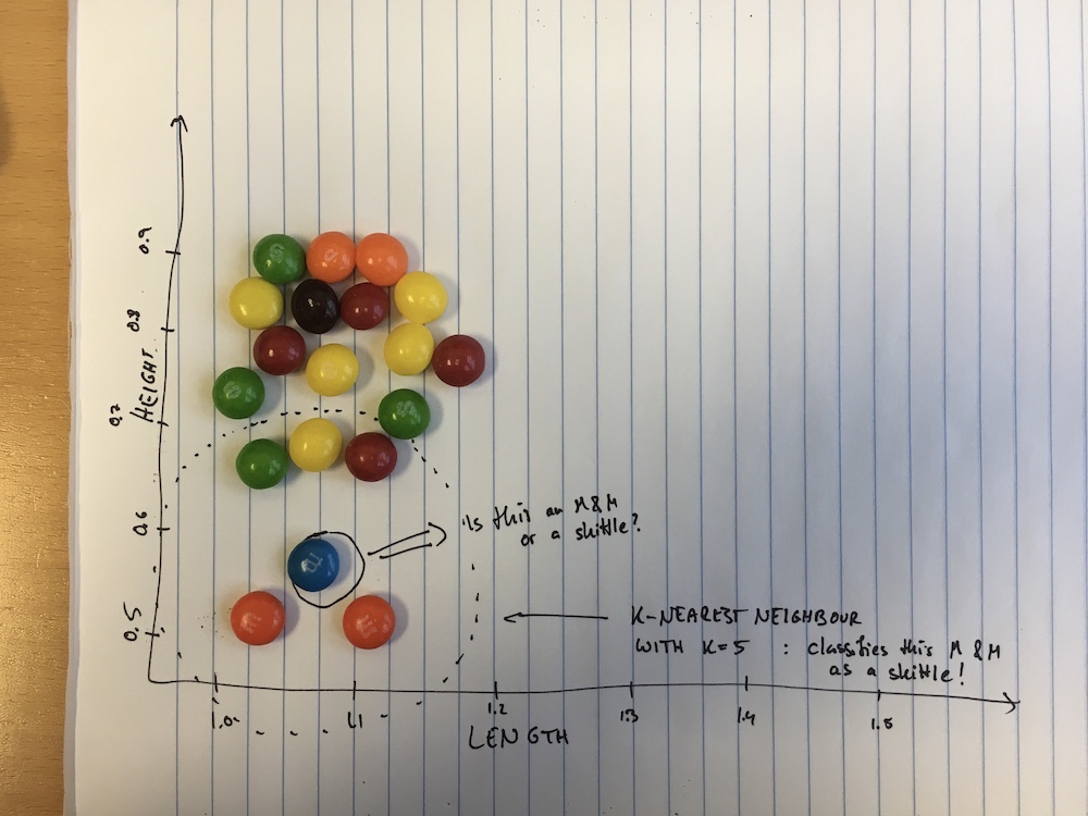
Let’s take a look at my version of this challenge:

Here I’ve made a graph of the length (the widest extent) and the height (the smallest extent). I used only skittles and plain M&Ms on the plot, because they’re quite similar in overall shape, but skittles tend to be thicker. I pretended that I only have two plain M&Ms in my training set and many more skittles. I then took another candy (the blue one circled on the figure) and placed it on the graph according to its height and length. This new candy seems to be much closer to the two M&Ms than it is to any of the skittles, so we might assume that it’s an M&M, too. In order to use our K-Nearest Neighbour algorithm with $k = 1$, we look for the closest candy already on the plot: one of the orange ones, which seem to be about equidistant from our blue one. Both of these are M&Ms, so with k=1 (and, indeed k=2) our conclusion stays the same.

Now what happens if I increase k? Let’s try for k=5.
The five closest to my blue one still contain the two M&Ms, but they now also contain three skittles (the green, yellow and red ones on the figure above)! We would now conclude that actually, our candy is a skittle not an M&M!

What happened here? Well, we fell into a common pitfall of machine learning: if our training data (the we placed on the graph for which we know what they are) is very imbalanced, that is if I have many more of one type (skittles) than the other (M&Ms), a machine learning algorithm might ignore the existance of examples of the smaller class (here the M&Ms) entirely. Notice how no matter where you’d place a candy on the graph, if k = 5 or above, the algorithm will always conclude that the candy we placed is a skittle, because for any candy the number of M&Ms that are closest is at most two, and the number of nearby skittles must always be at least three or above.

So when you’re doing machine learning, beware of imbalanced training data sets! We will explore this more later in the lesson.

The Mathematics of K-Nearest Neighbour

Let’s look a little closer at how we can calculate our k-nearest neighbour results in practice.

For this, we’re going to formalize our previous intuitions with some maths. Assume you have training examples $\{X_1, X_2, X_3, ... X_n\}$, where each $X_i$ is a vector of features (like length, height, colour etc.) and associated labels $\{y_1, y_2, y_3 ..., y_n\}$ (e.g. plain M&M, peanut M&M, skittle, …).

For a given new unknown example $<X_u, y_u>$, we compute a distance function $d(X_u, X_i)$ between our new example and all training examples. There are a number of different distance functions one can use. A commonly used one is the Euclidean distance,

Assuming we have computed the distance between our unknown example and all training examples we can select the set $D_k = \{ <X_1, y_1>, <X_2, y_2>, ..., <X_k, y_k> \}$ of $k$ nearest neighbours (examples with the smallest distance). We can now compute the conditional probability for each class (i.e. the fraction of points in $D_k$ with a given class label):

where $I$ is the indicator function ($I = 1$ if $i=j$, else $I = 0$).

Advanced Challenge

In this challenge, we are going to write our own implementation of the k-nearest neighbours algorithm!

1) First, download the data from the GitHub repository. 2) Load this data in whatever programming environment you use for data analysis (I use Python, so I would use the Pandas library to load it). 3) Separate out the first two thirds and the last third of the table into separate tables. The first table with most of the data will be our designated training data. For the second table, we’ll assume that we don’t know the labels. This’ll be our target data, which we’d like to classify. 4) Then, for each of our training and target data, store the features in a separate array from the labels. 5) Write a function that takes two examples and calculates the Euclidean distance defined above between them. 6) Calculate the distances between the first example in your target data, and all examples in your training data. 7) Copy your array of class labels for your training data, and then order this array by the distances you just derived (so that the label associated to the example with the smallest distance is first, the one with the second-smallest distance next, etc.) 8) Out of this array, you can now pick the first $k$ examples for a varying number of $k$. Try with $k = 1, 2, 5, 10, 20$, and for each count the occurrence rates of the different class labels.

Assuming that we pick the class for our example that corresponds to the highest number of training examples out of our $k$ nearest neighbours, how does the prediction for your chosen target example change as you increase $k$? Does the algorithm predict your example accurately?

Solution

Need to write solution in Python.

Key Points