Logistic Regression

Overview

Teaching: 20 (+20) min
Exercises: 20 (+60) min

Questions

• How can we get a computer to draw decision boundaries between different types of candies?

Objectives

• Learners develop an intuition about logistic regression as a way to model two-class problems.

• More advanced learners can also write their own version of the algorithm in code, and use the data they generated to classify new data points.

K-Nearest Neighbours is just one out of many different machine learning algorithms (there’ll be some resources for further reading at the end of the tutorial). Let’s take a look at a second, very different algorithm, to get a feeling for how different algorithms work.

For this particular algorithm, we’re going to simplify the initial problem. We’re going to try to distinguish plain M&Ms from peanut M&Ms only, and we’re going to look at a single feature: the longest extent of each candy, which I’ve labelled “length” in my data set.

To prepare we’re also going to make one change in our data set. When I recorded my measurements, I wrote down what each candy I measured was in words, e.g. “plain M&M”, and “peanut M&M”. This is great, because it’s descriptive! However, for this algorithm to work, we’re going to need to transform our labels into numbers, so we’re going to do a substitution. Plain M&Ms will be labelled with “0”, peanut M&Ms will be labelled with “1” (the reason for these numbers will become clear in a moment). Once we’ve done that, we can now plot the data for our plain and peanut M&Ms on a graph, like so:

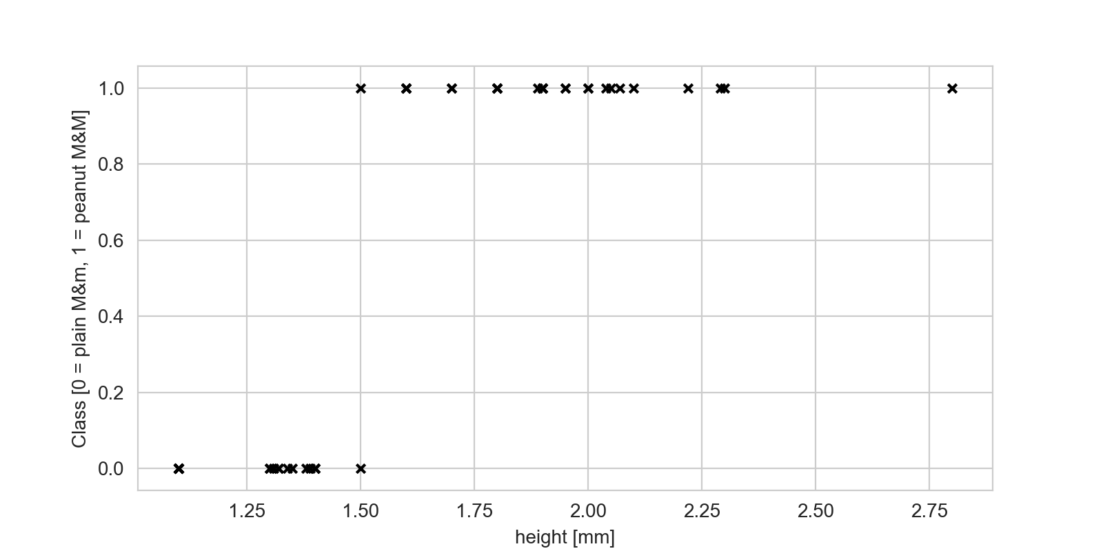
We can see that the plain M&Ms cluster to the left (all their points are zero on the y-axis), whereas the peanut M&Ms cluster to the right. This is because the peanut M&Ms have, well, peanuts in them, so they’re longer. What we want to do is predict whether a given piece of candy is a plain or peanut M&M, given that we’ve measured its length. In order to do that, we want to fit a function through our data points. If we can find a function that describe our data points well, then for any given length we measured from an unknown piece of candy, we can read the relevant label off that function.

Challenge

Make a sketch of the graph above on some paper (it doesn’t have to be very precise, just a rough approximation. Can you come up with a function that might fit through these data points?

Solution

The simplest function we could fit through these data points is a step function, which will predict zeros for all heights below a certain threshold, and ones above:

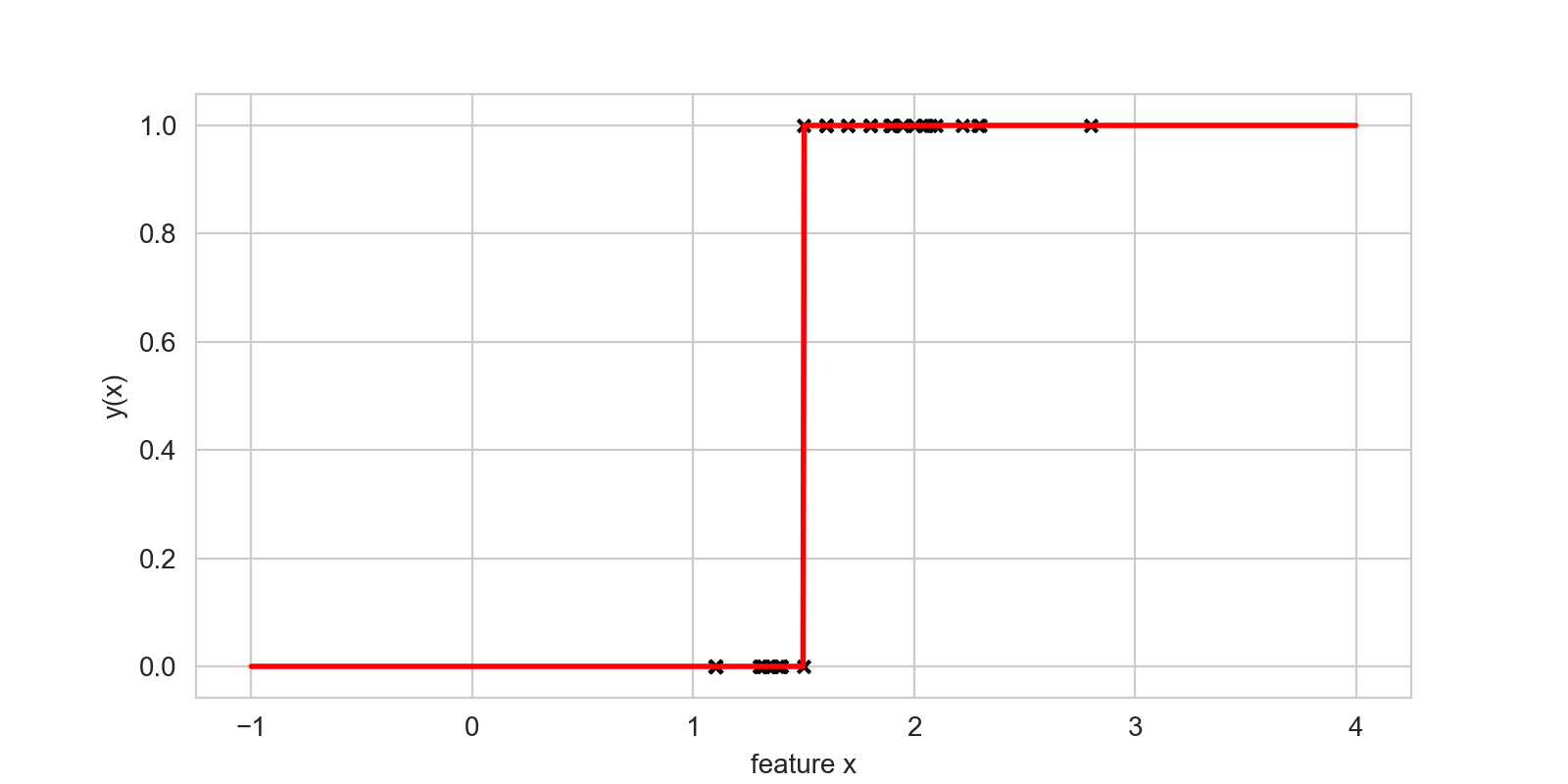
While the step function mentioned in the solution to the challenge above does really well at modelling this problem, it has some undesirable characteristics: in particular, because it has a discontinuity at the threshold, it is not differentiable, which makes optimization (i.e. using a computer to find the best value for that threshold), difficult in practice.

So what is the simplest differentiable model we could use? Well, the simplest model is a straight line, $z = ax + b$ so let’s fit that through our data:

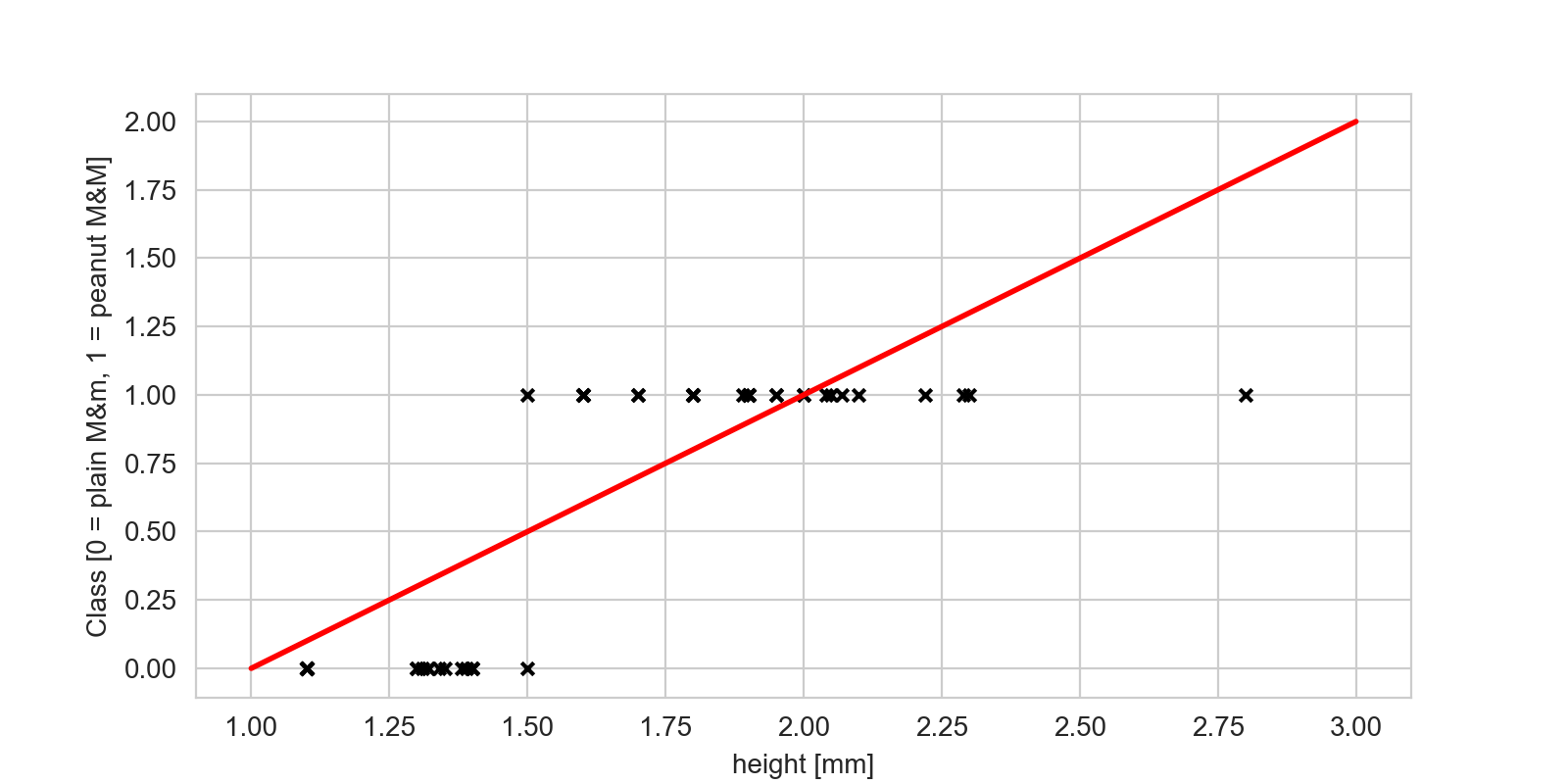
That’s a simpler model, but not one that fits our data particularly well; the function does not really go through the data points. The reason is that the straight line model predicts a real value $z$ for each input $x$ (the measured length feature), but our outputs aren’t continuous real values — they’re either zeros or ones! There’s a trick we can employ to take that straight line model above, and make it output mostly zeros and ones, and produce a function that is quite similar to the step function we used above.

This is called the logistic function, which is defined as

So if we have a single feature (length), as defined above, our predicted outputs become

What does this function look like for $a=1$ and $b=0$?

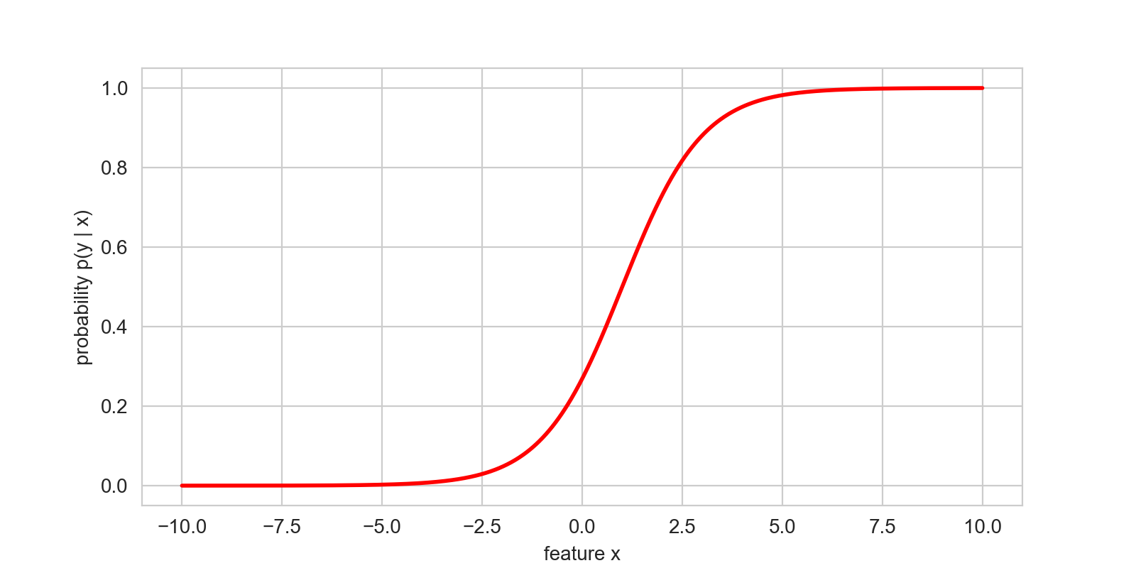
By default, the logistic function is 0 for $x << 0$, 1 for $x >> 0$, and crosses $0.5$ exactly at $x = 0$. We can find some reasonable values for $a$ and $b$ (in the challenge below, you’ll get to do that yourself on a computer), and see whether we can make this model fit through the data:

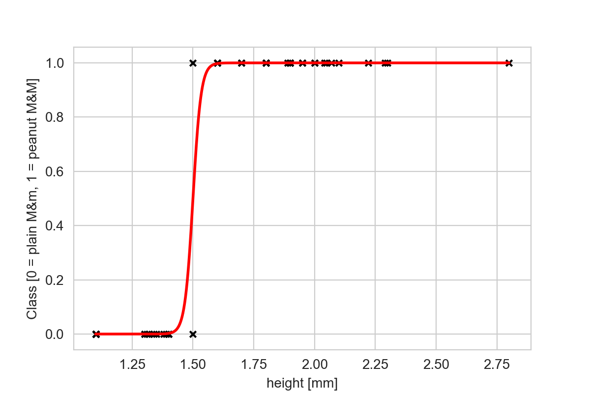
Overall this does much better than the straight line at fitting through our data points, though it doesn’t quite as well as the step function. If you look closely, you can see that in my data set there’s at least one peanut M&M and one plain M&M that have the same recorded length of 1.5cm. This means that with this single feature, it is impossible to distinguish whether your candy is a plain or peanut M&M if it’s exactly 1.5cm long.

If our candies have lengths that are far away 1.5cm, then the function will predict values close to either 0 or 1, and we can confidently predict that the candies are either plain or peanut. However, if the length you’ve measured is close to 1.5 then the function will predict something close to 0.5, making it nearly impossible to safely classify.

Challenge

Discuss with a neighbour: what should you conclude if you measure a height close to 1.5cm? Can you think of ways to interpret the fact that the model doesn’t jump from 0 to 1 in the same way as the step function, but has values in between for certain values of your feature?

Solution

In many standard applications, the creators of the model define 0.5 as a hard cut-off: any predictions of values smaller than 0.5 are assumed to belong to samples belonging to class 0, and all predictions with values larger than 0.5 belong to class 1. In some way, one reproduces the result of the step function model above, but with nicer mathematical properties.

However, in the process, you loose some valuable information. Statistically, the logistic regression model calculates the probability that the class of a sample is 1, given some measurement $x$, $P(y = 1 | x)$. If the feature is very small, the logistic model predicts 0 or near-zero values, suggesting that the probability that a sample with that feature value belongs to class 1 (peanut M&Ms). Conversely, for large values of the feature, the logistic model predicts a value close to 1, suggesting that it’s pretty probable that the sample in question is a peanut M&M. For cases in the middle, the probability is close to 0.5, which means that the model really isn’t sure. This is expected, and in some way desirable: as we can see from our training data, there’s at least one instance where we have a peanut and a plain M&M with the same length. Based on that feature alone, we can therefore not confidently conclude that a sample is either one or the other.

Here, logistic regression gives you valuable information about how confident you can be about your prediction, which is helpful in many circumstances.

Logistic Regression Returns Probabilities

By default, logistic regression does not directly predict whether a given sample belongs to class 0 or class 1; it returns the probability that a sample might belong to class 1. As the person building the model, you still have to decide how to interpret that number for the purpose of classification. Keeping the information about probabilities can be very valuable, because even after you decide how you want to use these probabilities for classification, they give you helpful information about how confident you can be in your conclusions.

Challenge

In the previous challenge, we said that typically, model builders will set a threshold at a predicted value of 0.5. That is a deliberate choice, and you could make a different one!

Can you think of situations where 0.5 might not be a good threshold? Think back to our discussion about ethics, and some of the reasons for why we want to separate out peanut M&Ms and plain M&Ms in the first place. What other threshold would you implement, and why?

Solution

In our episode on ethics earlier, we talked about our friends with peanut-allergies, and how making a mistake in our classification might have serious health consequences if one of these friends accidentally ate a peanut M&M misclassified as a different type of candy. Protection our friends is really important; we don’t want to missclassify any peanut M&M’s as plain ones, whereas misclassifying a plain M&M as a peanut M&M is less severe.

Thus, we could consider setting the threshold at a much higher value. Perhaps as high as 0.999. In this case, many plain M&Ms might get misclassified as peanut M&Ms, but only one in a thousand peanut M&Ms should get misclassified as a plain M&M. That seems much safer!

As we have said in the ethics lesson, it is important to always check your assumptions and consider the possibly unintended, harmful outcomes of making mistakes in your classification.

Advanced Challenge

In this challenge, we are going to write our own implementation of the logistic regression algorithm!

1. First, download the data from the GitHub repository.
2. Load this data in whatever programming environment you use for data analysis (I use Python, so I would use the Pandas library to load it).
3. Take all rows that are either peanut or plain M&Ms, and store only those rows in a separate table (you can also pick another combination of two types of candy).
4. Separate out the first two thirds and the last third of the new table into separate tables. The first table with most of the data will be our designated training data. For the second table, we’ll assume that we don’t know the labels. This’ll be our target data, which we’d like to classify.
5. Then, for each of our training and target data, extract out a single feature (you can use length like I’ve done, or pick a different one.
6. For each of our training and target data, store the features in a separate array from the labels.
7. Rename the labels such that plain M&Ms are zeros, and peanut M&Ms are ones.
8. Write a function that, given a feature and parameters $a$ and $b$, calculates a straight line (linear model), then squashes that straight line through a logistic function.
9. Plot your feature (e.g. the length), and plot a standard logistic function (with $a=1$ and $b=0$).
10. Play around with $a$ and $b$ until you find values that match our data set, note those values down, and compare with your neighbours.
11. For a given height
12. Copy your array of class labels for your training data, and then order this array by the distances you just derived (so that the label associated to the example with the smallest distance is first, the one with the second-smallest distance next, etc.)
13. Out of this array, you can now pick the first $k$ examples for a varying number of $k$. Try with $k = 1, 2, 5, 10, 20$, and for each count the occurrence rates of the different class labels.

Multiple Features

How can we handle multiple features?

In the example data set, I’ve collected features for length, height, width, colour, and others. We can include these extra features by adding more parameters and dimensions to our linear model. For example, for two features $x_1$ and $x_2$ (e.g. length and height), we can write down a linear model

which we can then use as input into the logistic function in the same way we’ve done above. Here, $a_1$ and $a_2$ are now two different parameters, which need to be estimated simultaneously.

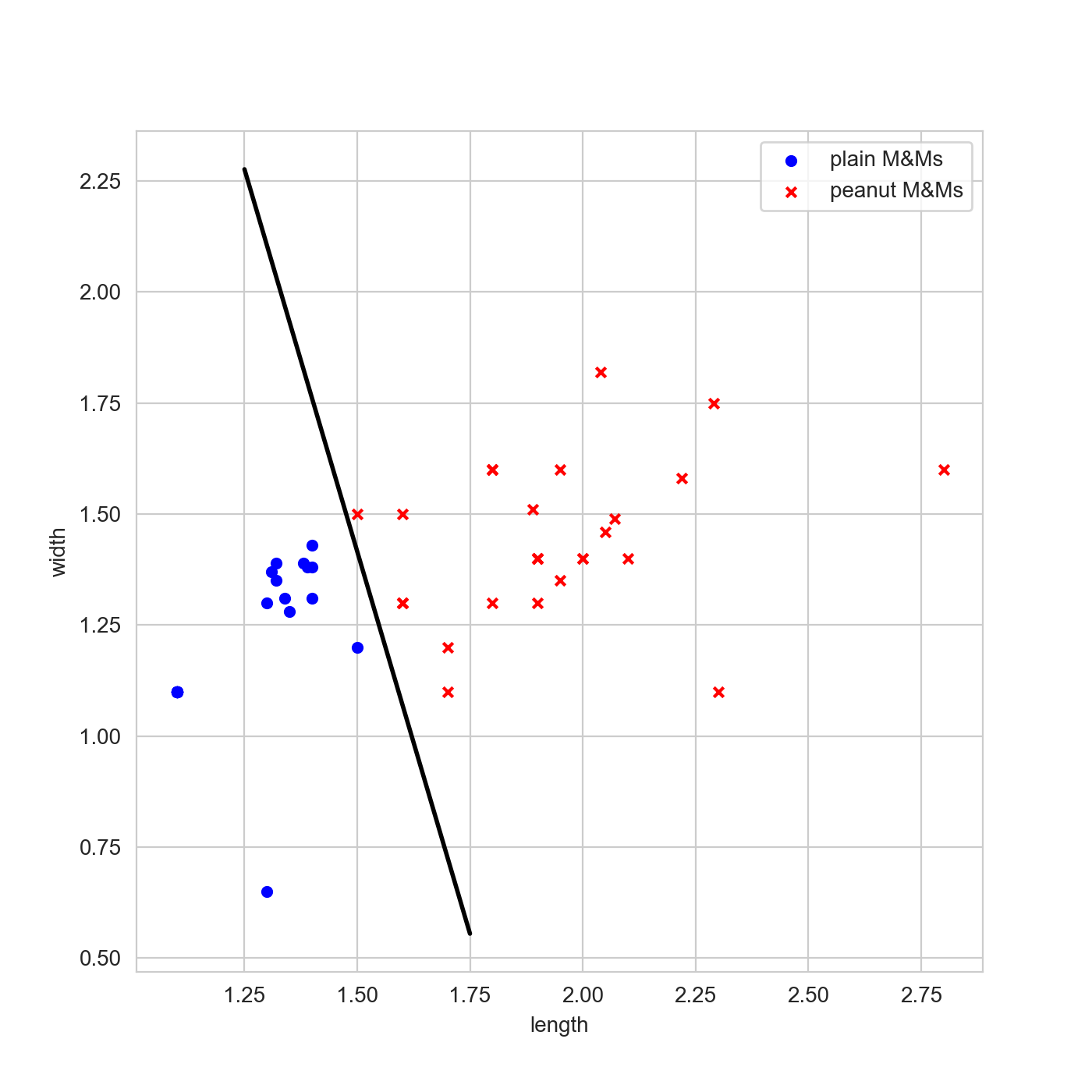
This is a bit harder to represent visually, because we have added a dimension. Instead of plotting feature versus outcome we are going to plot feature versus feature, where I’ve used different colours and symbols for the different classes. Instead of plotting the predictions as we’ve done above, I’m also going to set the threshold for decision between the classes at 0.5, and plot the $\sigma(z) = 0.5$ contour. This is, for this case, the decision boundary.

Challenge

Where on the plot are the two samples that had the same length? Are they easier to distinguish now?

Solution

If you look closely, the two points at a length of 1.5 are separated quite well in width: the plain M&M is just below 1.25cm in width, and the peanut M&M is about 1.5cm in width. Adding more descriptive features can help us separate out different classes better! However, it’s also worth checking whether the new features you include actually help you separate out different classes better, or just add noise.

Plot Your Features

Plotting different features against one another can help you learn about which features might improve your classification, and which ones won’t. A useful visualization for this purpose is called a scatterplot matrix (also called a pairs plot or a corner plot).

Key Points

• Logistic regression is an extension to linear regression models that allows for modelling problems where the outcomes are 0 and 1.

• Logistic regression allows for separation of two different classes via a decision boundary.